Binary State Speciation and Extinction Model: Split Models

Create a likelihood function for a BiSSE model where the tree is partitioned into regions with different parameters. Alternatively, make.bisse.uneven can be used where different regions of the tree have different fractions of species known.

make.bisse.split(tree, states, nodes, split.t, unresolved=NULL,
                 sampling.f=NULL, nt.extra=10, strict=TRUE, control=list())
make.bisse.uneven(tree, states, nodes, split.t, unresolved=NULL,
                  sampling.f=NULL, nt.extra=10, strict=TRUE, control=list())

Arguments

tree: An ultrametric bifurcating phylogenetic tree, in ape “phylo” format.
states: A vector of character states, each of which must be 0 or 1, or NA if the state is unknown. This vector must have names that correspond to the tip labels in the phylogenetic tree (tree$tip.label). For tips corresponding to unresolved clades, the state should be NA.
nodes: Vector of nodes that will be split (see Details).
split.t: Vector of split times, same length as nodes (see Details).
unresolved: Unresolved clade information: see section below for structure.
sampling.f: Vector of length 2 with the estimated proportion of extant species in state 0 and 1 that are included in the phylogeny. A value of c(0.5, 0.75) means that half of species in state 0 and three quarters of species in state 1 are included in the phylogeny. By default all species are assumed to be known. Alternatively, with split models this can be a list of length (length(nodes) + 1), each element of which is a vector of length 2. The first element is the sampling fraction for the “background” group, the second element corresponds to the clade subtended by nodes[1], and the ith element corresponding to the clade subtended by nodes[i+1].
nt.extra: The number of species modelled in unresolved clades (this is in addition to the largest observed clade).
strict: The states vector is always checked to make sure that the values are 0 and 1 only. If strict is TRUE (the default), then the additional check is made that every state is present. The likelihood models tend to be poorly behaved where states are missing.
control: List of control parameters for the ODE solver. See details in make.bisse.

Details

Branching times can be controlled with the split.t argument. If this is Inf, split at the base of the branch (as in MEDUSA). If 0, split at the top (closest to the present, as in the new option for MEDUSA). If 0 < split.t < Inf then we split at that time on the tree (zero is the present, with time growing backwards).

TODO: Describe nodes and split.t here.

Author

Richard G. FitzJohn

Examples

## Due to a change in sample() behaviour in newer R it is necessary to
## use an older algorithm to replicate the previous examples
if (getRversion() >= "3.6.0") {
  RNGkind(sample.kind = "Rounding")
}
#> Warning: non-uniform 'Rounding' sampler used

pars <- c(0.1, 0.2, 0.03, 0.03, 0.01, 0.01)
set.seed(546)
phy <- tree.bisse(pars, max.taxa=30, x0=0)

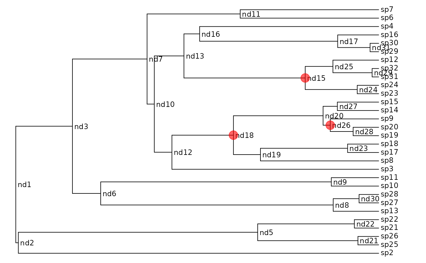
## Here is the phylogeny:
plot(phy, show.node.label=TRUE, label.offset=.1, font=1, cex=.75,
     no.margin=TRUE)

## Here is a plain BiSSE function for comparison:
lik.b <- make.bisse(phy, phy$tip.state)
lik.b(pars) # -93.62479
#> [1] -93.62479

## Split this phylogeny at three points: nd15, nd18 and nd26
nodes <- c("nd15", "nd18", "nd26")

## This is the index in ape's node indexing:
nodes.i <- match(nodes, phy$node.label) + length(phy$tip.label)

nodelabels(node=nodes.i, pch=19, cex=2, col="#FF000099")


## To make a split BiSSE function, pass the node locations and times in:
lik.s <- make.bisse.split(phy, phy$tip.state, nodes.i)

## The parameters must be a list of the same length as the number of
## partitions.  Partition '1' is the root partition, and partition i is
## the partition rooted at the node[i-1]
pars4 <- rep(pars, 4)
pars4
#>  [1] 0.10 0.20 0.03 0.03 0.01 0.01 0.10 0.20 0.03 0.03 0.01 0.01 0.10 0.20 0.03
#> [16] 0.03 0.01 0.01 0.10 0.20 0.03 0.03 0.01 0.01

## Run the likelihod calculation:
lik.s(pars4) # -93.62479
#> [1] -93.62479

## These are basically identical (to acceptable tolerance)
lik.s(pars4) - lik.b(pars)
#> [1] -1.397798e-08

## You can use the labelled nodes rather than indices:
lik.s2 <- make.bisse.split(phy, phy$tip.state, nodes)
identical(lik.s(pars4), lik.s2(pars4))
#> [1] TRUE