integrate_const. rodeint 0.1

Usage

integrate_const(stepper, ode_system, y, t0, t1, dt, save_state = FALSE)
integrate_n_steps(stepper, ode_system, y, t0, dt, n, save_state = FALSE)
integrate_adaptive(stepper, ode_system, y, t0, t1, dt, save_state = FALSE)
integrate_times(stepper, ode_system, y, times, dt)

Arguments

stepper: A stepper object, created by make_stepper
ode_system: A system of ODEs, created by ode_system
y: Initial conditions
t0: Time to start the integration
t1: Time to finish the integration
dt: Step size
n: Number of steps to take (integrate_n_steps only)
times: Vector of times (integrate_times only)
save_state: Logical: return information about intermediate points as an attribute. Not applicable for integrate_times, which always returns information about intermediate points.

Integrate a System of ODEs

Description

Integrate a system of ordinary differential equations (ODEs). This is the low-level interface that corresponds exactly to the ideint interface. An easier to use, more R-ish, interface is available using make_integrate.

Details

There are four different integration functions here. See the odeint documentation for more detail about the precice differences. The summary, though, is:

integrate_const "Equidistant observer calls"
integrate_n_steps "Integrate a given number of steps"
integrate_adaptive "Observer calls at each step"
integrate_times "Observer calls at given time points"

This page provides much more detail. The functions here are direct wrappers of the odeint functions, so the interpretation is identical.

If you just want the end-points, integrate_adaptive is probably the function to use. If you want to know intermediate values at particular times too, use integrate_times. The functions integrate_const and integrate_n_steps are provided more for completeness than for utility, but they may be useful in specific applications.

Examples

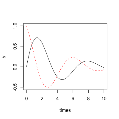
## Picking up with the harmonic oscillator from the ode_system
## example:
derivs <- function(y, t, pars) {
  c(y[2],
    -y[1] - pars * y[2])
}

## Parameters of the system:
pars <- 0.5

## Build the system itself
sys <- ode_system(derivs, pars)

## We also need a stepper (see the ?stepper help page)
s <- make_stepper("dense", "runge_kutta_dopri5")

## Suppose we want output at these times:
times <- seq(0, 10, length=101)

## Starting from this initial state:
y0 <- c(0, 1)

## Initial step size guess:
dt <- 0.01

## This intergrates the system (all integrate_ functions take stepper,
## system, y as the first theree arguments).
y <- integrate_times(s, sys, y0, times, dt)

## Here are the variables changing over time:
matplot(times, y, type="l")



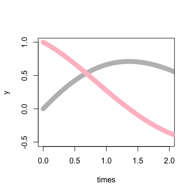
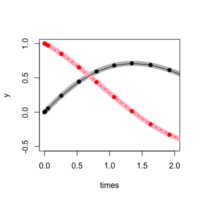
## The result also has useful attributes.  The "t" attribute is the
## times (this is the same as 'times' here)
attr(y, "t")

  [1]  0.0  0.1  0.2  0.3  0.4  0.5  0.6  0.7  0.8  0.9  1.0  1.1  1.2  1.3  1.4
 [16]  1.5  1.6  1.7  1.8  1.9  2.0  2.1  2.2  2.3  2.4  2.5  2.6  2.7  2.8  2.9
 [31]  3.0  3.1  3.2  3.3  3.4  3.5  3.6  3.7  3.8  3.9  4.0  4.1  4.2  4.3  4.4
 [46]  4.5  4.6  4.7  4.8  4.9  5.0  5.1  5.2  5.3  5.4  5.5  5.6  5.7  5.8  5.9
 [61]  6.0  6.1  6.2  6.3  6.4  6.5  6.6  6.7  6.8  6.9  7.0  7.1  7.2  7.3  7.4
 [76]  7.5  7.6  7.7  7.8  7.9  8.0  8.1  8.2  8.3  8.4  8.5  8.6  8.7  8.8  8.9
 [91]  9.0  9.1  9.2  9.3  9.4  9.5  9.6  9.7  9.8  9.9 10.0


## The "steps" attributes contains the number of steps the system took
attr(y, "steps")

[1] 34


## Here, the number is lower than the number of times!  This is
## because we used a "dense output stepper" which can interpolate back
## over times that have passed.  See the "See also" section for a link
## to the odeint help about this.

## The "y" attribute contains the final system state - here it will be
## the same as the last row of 'y' itself
attr(y, "y")

[1] -0.02160347 -0.07397367

y[nrow(y),]

[1] -0.02160347 -0.07397367


## If you don't care about intermediate times, the
## "integrate_adaptive" function is probably the right one to use.
y_a <- integrate_adaptive(s, sys, y0, min(times), max(times), dt)
y_a

[1] -0.02160347 -0.07397367


## Here we jump all the way to the final time as quickly as possible.
y_a

[1] -0.02160347 -0.07397367

attr(y, "y")

[1] -0.02160347 -0.07397367


## It's possible to remember the steps taken by usin the "save_state"
## argument.
y_a <- integrate_adaptive(s, sys, y0, min(times), max(times), dt,
                          save_state=TRUE)

## Now y_a contains three attributes, the same as returned by
## integrate_times.  "t" is the vector of times that the stepper
## stopped at:
attr(y_a, "t")

 [1]  0.0000000  0.0100000  0.0550000  0.2575000  0.5286291  0.7997582
 [7]  1.0708873  1.3420164  1.6309726  1.9199289  2.2088851  2.4978413
[13]  2.7867975  3.0757537  3.3769160  3.6780782  3.9792404  4.2804026
[19]  4.5815649  4.9062149  5.2308649  5.5555149  5.8801650  6.2048150
[25]  6.5294650  6.8677236  7.2059821  7.5442406  7.8969110  8.2710404
[31]  8.6451698  9.0192992  9.3934286  9.7675581 10.0000000


## "y" contains the y values at these points, wherever they are:
attr(y_a, "y")

              [,1]         [,2]
 [1,]  0.000000000  1.000000000
 [2,]  0.009974875  0.994962646
 [3,]  0.054223288  0.971390003
 [4,]  0.238952009  0.848922710
 [5,]  0.443225135  0.653105633
 [6,]  0.591317282  0.437489651
 [7,]  0.680232383  0.219316983
 [8,]  0.711397537  0.013818617
 [9,]  0.686939264 -0.177312376
[10,]  0.612736126 -0.329041820
[11,]  0.501208969 -0.434955990
[12,]  0.365989311 -0.493041141
[13,]  0.220704048 -0.505247071
[14,]  0.077924018 -0.476803382
[15,] -0.056715101 -0.412187698
[16,] -0.167793270 -0.322159984
[17,] -0.249321789 -0.217795884
[18,] -0.298618473 -0.109820786
[19,] -0.316069565 -0.007762507
[20,] -0.302701104  0.086826934
[21,] -0.262144225  0.158870217
[22,] -0.202383887  0.204797941
[23,] -0.132060540  0.224094028
[24,] -0.059538647  0.218887991
[25,]  0.007858600  0.193353173
[26,]  0.066468459  0.151073056
[27,]  0.109028144  0.099619884
[28,]  0.133597519  0.045785838
[29,]  0.140335725 -0.006429422
[30,]  0.129061730 -0.051716116
[31,]  0.103426366 -0.082750940
[32,]  0.069114475 -0.098049484
[33,]  0.031935795 -0.098366179
[34,] -0.002929415 -0.086217132
[35,] -0.021603470 -0.073973666


## Here is the dense output (thick lines) with the actual observed
## spots overlaid.  You can see the step size change at the beginning
## of the problem until the stepper works out how fast it can go while
## achieving the required accuracy.
matplot(times, y, type="l", col=c("grey", "pink"), lty=1, lwd=10,
        xlim=c(0, 2))


matlines(attr(y_a, "t"), attr(y_a, "y"), type="o", pch=19)



## Manually specifying the stepper and step size and passing around 6
## or so parameters all the time gets old, so there is a function
## "make_integrate" to help collect everything together.  See
## ?make_integrate for more information.

Author

Rich FitzJohn